Modeling
Modeling
The Core Modeling Decisions
What architecture should the model follow? How many parameters should it have? These decisions impact not only the model's capabilities but also its usability for downstream applications.
Deployment Footprint
Latency Strategy
Design Tradeoffs
Model Architecture
As of this writing, the most dominant architecture for language-based foundation models is the transformer architecture (Vaswani et al., 2017), which is based on the attention mechanism. It addresses many limitations of previous architectures, which contributed to its popularity.
Transformer Architecture
To understand the transformer, let's look at the problem it was created to solve. The transformer architecture was popularized on the heels of the success of the seq2seq (sequence-to-sequence) architecture. At the time of its introduction in 2014, seq2seq provided significant improvement on then-challenging tasks: machine translation and summarization.
In 2016, Google incorporated seq2seq into Google Translate, an update that they claimed to have given them the "largest improvements to date for machine translation quality". This generated a lot of interest in seq2seq, making it the go-to architecture for tasks involving sequences of text.
Encoder
Decoder
Both inputs and outputs are sequences of tokens, hence the name. Seq2seq uses RNNs (recurrent neural networks) as its encoder and decoder. A visualization of the seq2seq architecture is shown in the top half of Figure 2-4.
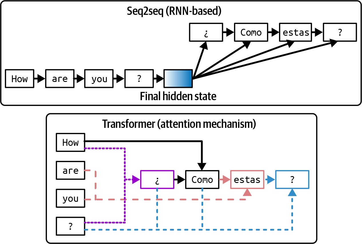
Figure 2-4. Seq2seq architecture versus transformer architecture. For the transformer architecture, the arrows show the tokens that the decoder attends to when generating each output token.
The Two Seq2seq Bottlenecks
There are two problems with seq2seq that Vaswani et al. (2017) addresses.
Final-State Bottleneck
Sequential Processing
The transformer architecture addresses both problems with the attention mechanism. The attention mechanism allows the model to weigh the importance of different input tokens when generating each output token. This is like generating answers by referencing any page in the book. A simplified visualization of the transformer architecture is shown in the bottom half of Figure 2-4.
The transformer architecture dispenses with RNNs entirely. With transformers, the input tokens can be processed in parallel, significantly speeding up input processing. While the transformer removes the sequential input bottleneck, transformer-based autoregressive language models still have the sequential output bottleneck.
Inference Has Two Steps
Inference for transformer-based language models consists of two steps:
Prefill
Decode
Attention Mechanism
At the heart of the transformer architecture is the attention mechanism. Understanding this mechanism is necessary to understand how transformer models work. Under the hood, the attention mechanism leverages key, value, and query vectors:
Query Vector (Q)
Key Vector (K)
Value Vector (V)
The attention mechanism computes how much attention to give an input token by performing a dot product between the query vector and its key vector. A high score means that the model will use more of that page's content (its value vector) when generating the book's summary.
A visualization of the attention mechanism with the key, value, and query vectors is shown in Figure 2-5. In this visualization, the query vector is seeking information from the previous tokens How, are, you, ?, ¿ to generate the next token.
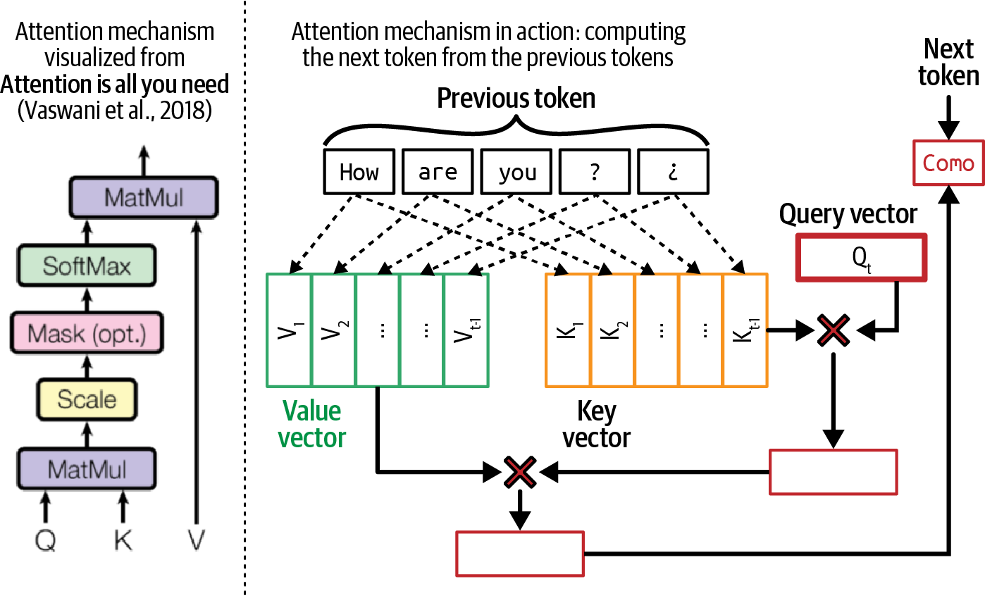
Figure 2-5. An example of the attention mechanism in action next to its high-level visualization from the famous transformer paper, "Attention Is All You Need" (Vaswani et al., 2017).
Attention Math
Let's look into how the attention function works. Given an input x, the key, value, and query vectors are computed by applying key, value, and query matrices to the input. Let , , and be the key, value, and query matrices. The key, value, and query vectors are computed as follows:
The query, key, and value matrices have dimensions corresponding to the model's hidden dimension. For example, in Llama 2-7B (Touvron et al., 2023), the model's hidden dimension size is 4096, meaning that each of these matrices has a 4096 x 4096 dimension. Each resulting K, V, Q vector has the dimension of 4096.4
The attention mechanism is almost always multi-headed. Multiple heads allow the model to attend to different groups of previous tokens simultaneously.
K, V, and Q vector will be split into 32 vectors of the dimension 128. This is because 4096 / 32 = 128.The outputs of all attention heads are then concatenated. An output projection matrix is used to apply another transformation to this concatenated output before it's fed to the model's next computation step. The output projection matrix has the same dimension as the model's hidden dimension.
Transformer Block
Now that we've discussed how attention works, let's see how it's used in a model. A transformer architecture is composed of multiple transformer blocks. The exact content of the block varies between models, but, in general, each transformer block contains the attention module and the MLP (multi-layer perceptron) module:
Attention Module
MLP Module
Common nonlinear functions are ReLU, Rectified Linear Unit (Agarap, 2018), and GELU (Hendrycks and Gimpel, 2016), which was used by GPT-2 and GPT-3, respectively. Activation functions are very simple.5 For example, all ReLU does is convert negative values to 0. Mathematically, it's written as:
The number of transformer blocks in a transformer model is often referred to as that model's number of layers. A transformer-based language model is also outfitted with a module before and after all the transformer blocks:
Embedding Module
Output Layer
Figure 2-6 visualizes a transformer model architecture. The size of a transformer model is determined by the dimensions of its building blocks.
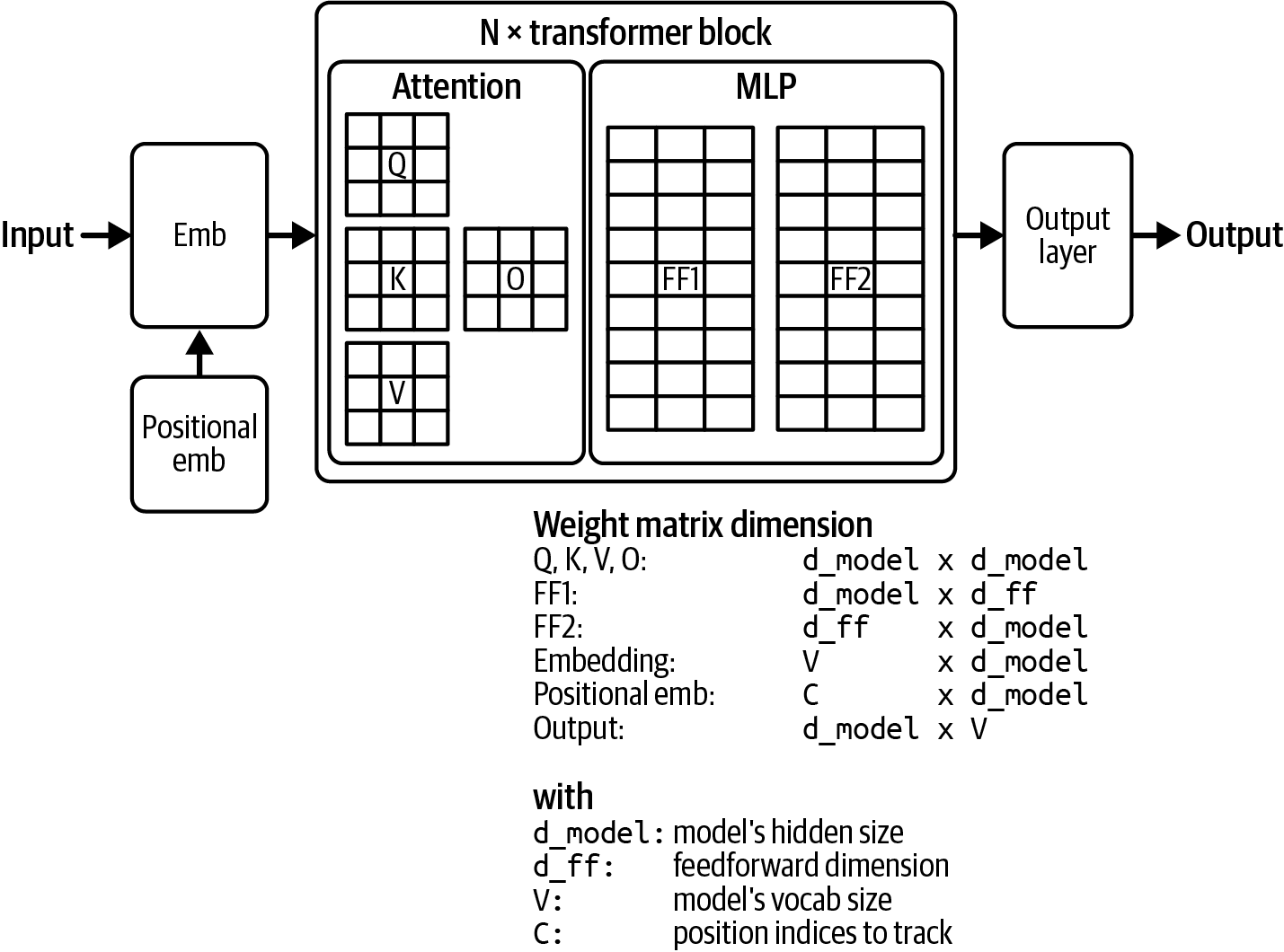
Figure 2-6. A visualization of the weight composition of a transformer model.
Larger dimension values result in larger model sizes. Table 2-4 shows these dimension values for different Llama 2 (Touvron et al., 2023) and Llama 3 (Dubey et al., 2024) models. Note that while the increased context length impacts the model's memory footprint, it doesn't impact the model's total number of parameters.
Table 2-4. The dimension values of different Llama models.
| Model | # transformer blocks | Model dim | Feedforward dim | Vocab size | Context length |
|---|---|---|---|---|---|
| Llama 2-7B | 32 | 4,096 | 11,008 | 32K | 4K |
| Llama 2-13B | 40 | 5,120 | 13,824 | 32K | 4K |
| Llama 2-70B | 80 | 8,192 | 22,016 | 32K | 4K |
| Llama 3-7B | 32 | 4,096 | 14,336 | 128K | 128K |
| Llama 3-70B | 80 | 8,192 | 28,672 | 128K | 128K |
| Llama 3-405B | 126 | 16,384 | 53,248 | 128K | 128K |
Other Model Architectures
While the transformer model dominates the landscape, it's not the only architecture. Since AlexNet revived the interest in deep learning in 2012, many architectures have gone in and out of fashion. Seq2seq was in the limelight for four years (2014-2018). GANs (generative adversarial networks) captured the collective imagination a bit longer (2014-2019).
Compared to architectures that came before it, the transformer is sticky. It's been around since 2017.6 How long until something better comes along?
However, there's hope. While transformer-based models are dominating, as of this writing, several alternative architectures are gaining traction.
RWKV
State Space Models
Since the architecture's introduction in 2021, multiple techniques have been introduced to make SSMs more efficient, better at long sequence processing, and scalable to larger model sizes.
S4
S4, introduced in "Efficiently Modeling Long Sequences with Structured State Spaces" (Gu et al., 2021b), was developed to make SSMs more efficient.
H3
H3, introduced in "Hungry Hungry Hippos: Towards Language Modeling with State Space Models" (Fu et al., 2022), incorporates a mechanism that allows the model to recall early tokens and compare tokens across sequences. This mechanism's purpose is akin to that of the attention mechanism in the transformer architecture, but it is more efficient.
Mamba
Mamba, introduced in "Mamba: Linear-Time Sequence Modeling with Selective State Spaces" (Gu and Dao, 2023), scales SSMs to three billion parameters. On language modeling, Mamba-3B outperforms transformers of the same size and matches transformers twice its size. The authors also show that Mamba's inference computation scales linearly with sequence length, compared to quadratic scaling for transformers. Its performance shows improvement on real data up to million-length sequences.
Jamba
Jamba, introduced in "Jamba: A Hybrid Transformer-Mamba Language Model" (Lieber et al., 2024), interleaves blocks of transformer and Mamba layers to scale up SSMs even further. The authors released a mixture-of-experts model with 52B total available parameters (12B active parameters) designed to fit in a single 80 GB GPU. Jamba shows strong performance on standard language model benchmarks and long-context evaluations for up to a context length of 256K tokens. It also has a small memory footprint compared to vanilla transformers.
Figure 2-7 visualizes the transformer, Mamba, and Jamba blocks.
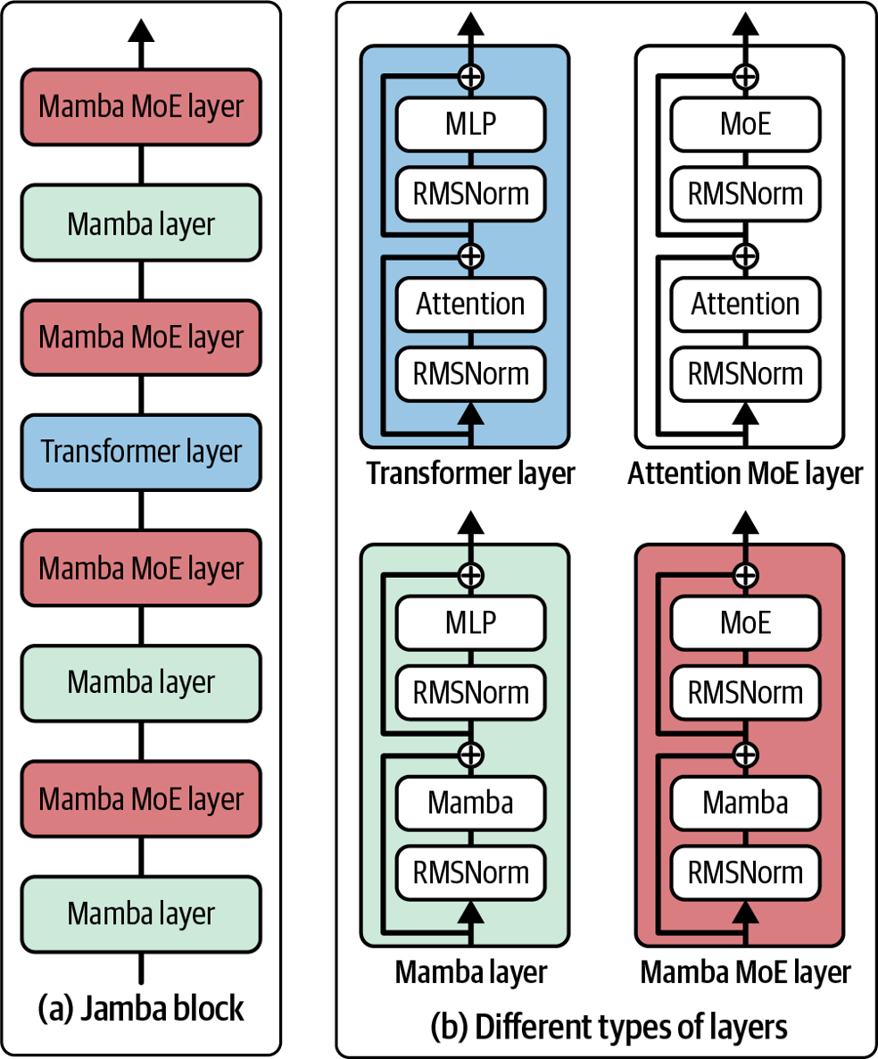
Figure 2-7. A visualization of the transformer, Mamba, and Jamba layers. Image adapted from "Jamba: A Hybrid Transformer-Mamba Language Model" (Lieber et al., 2024).
Model Size
Much of AI progress in recent years can be attributed to increased model size. It's hard to talk about foundation models without talking about their number of parameters. The number of parameters is usually appended at the end of a model name. For example, Llama-13B refers to the version of Llama, a model family developed by Meta, with 13 billion parameters.
In general, increasing a model's parameters increases its capacity to learn, resulting in better models. Given two models of the same model family, the one with 13 billion parameters is likely to perform much better than the one with 7 billion parameters.
The number of parameters helps us estimate the compute resources needed to train and run this model. For example, if a model has 7 billion parameters, and each parameter is stored using 2 bytes (16 bits), then we can calculate that the GPU memory needed to do inference using this model will be at least 14 billion bytes (14 GB).9
Sparse Models and MoE
The number of parameters can be misleading if the model is sparse. A sparse model has a large percentage of zero-value parameters. A 7B-parameter model that is 90% sparse only has 700 million non-zero parameters. Sparsity allows for more efficient data storage and computation. This means that a large sparse model can require less compute than a small dense model.
A type of sparse model that has gained popularity in recent years is mixture-of-experts (MoE) (Shazeer et al., 2017). An MoE model is divided into different groups of parameters, and each group is an expert. Only a subset of the experts is active for, or used to, process each token.
Total Parameters
Active Parameters
Dataset Size Matters Too
A larger model can also underperform a smaller model if it's not trained on enough data. Imagine a 13B-param model trained on a dataset consisting of a single sentence: "I like pineapples." This model will perform much worse than a much smaller model trained on more data.
When discussing model size, it's important to consider the size of the data it was trained on. For most models, dataset sizes are measured by the number of training samples. For example, Google's Flamingo (Alayrac et al., 2022) was trained using four datasets -- one of them has 1.8 billion (image, text) pairs and one has 312 million (image, text) pairs.
For language models, a training sample can be a sentence, a Wikipedia page, a chat conversation, or a book. A book is worth a lot more than a sentence, so the number of training samples is no longer a good metric to measure dataset sizes. A better measurement is the number of tokens in the dataset.
As of this writing, LLMs are trained using datasets in the order of trillions of tokens. Meta used increasingly larger datasets to train their Llama models:
Llama 1
1.4 trillion tokens for Llama 1
Llama 2
2 trillion tokens for Llama 2
Llama 3
15 trillion tokens for Llama 3
Together's open source dataset RedPajama-v2 has 30 trillion tokens. This is equivalent to 450 million books10 or 5,400 times the size of Wikipedia. However, since RedPajama-v2 consists of indiscriminate content, the amount of high-quality data is much lower.
See Table 2-5 for examples of the number of training tokens for models with different numbers of parameters.
Table 2-5. Examples of the number of training tokens for models with different numbers of parameters. Source: "Training Compute-Optimal Large Language Models" (DeepMind, 2022).
| Model | Size (# parameters) | Training tokens |
|---|---|---|
| LaMDA (Thoppilan et al., 2022) | 137 billion | 168 billion |
| GPT-3 (Brown et al., 2020) | 175 billion | 300 billion |
| Jurassic (Lieber et al., 2021) | 178 billion | 300 billion |
| Gopher (Rae et al., 2021) | 280 billion | 300 billion |
| MT-NLG 530B (Smith et al., 2022) | 530 billion | 270 billion |
| Chinchilla | 70 billion | 1.4 trillion |
Compute Requirements
Pre-training large models requires compute. One way to measure the amount of compute needed is by considering the number of machines, e.g., GPUs, CPUs, and TPUs. However, different machines have very different capacities and costs. An NVIDIA A10 GPU is different from an NVIDIA H100 GPU and an Intel Core Ultra Processor.
A more standardized unit for a model's compute requirement is FLOP, or floating point operation. FLOP measures the number of floating point operations performed for a certain task. Google's largest PaLM-2 model, for example, was trained using 10^22 FLOPs (Chowdhery et al., 2022). GPT-3-175B was trained using 3.14 x 10^23 FLOPs (Brown et al., 2020).
For example, an NVIDIA H100 NVL GPU can deliver a maximum of 60 TeraFLOP/s: 6 x 10^13 FLOPs a second or 5.2 x 10^18 FLOPs a day.12
1 FLOP/s-day = 60 x 60 x 24 = 86,400 FLOPsThis book uses FLOPs for counting floating point operations and FLOP/s for FLOPs per second.Assume that you have 256 H100s. If you can use them at their maximum capacity and make no training mistakes, it'd take you days, or approximately 7.8 months, to train GPT-3-175B.
However, it's unlikely you can use your machines at their peak capacity all the time. Utilization measures how much of the maximum compute capacity you can use. What's considered good utilization depends on the model, the workload, and the hardware.
Okay Utilization
Great Utilization
Chapter 9 discusses hardware metrics and utilization in more detail.
At 70% utilization and $2/h for one H100,13 training GPT-3-175B would cost over $4 million:
$2/H100/hour x 256 H100 x 24 hours x 256 days / 0.7 = $4,142,811.43
- Number of parameters, which is a proxy for the model's learning capacity.
- Number of tokens a model was trained on, which is a proxy for how much a model learned.
- Number of FLOPs, which is a proxy for the training cost.
$5,000 for each third prize, $20,000 for each second prize, and $100,000 for one first prize. They received a total of 99 submissions, of which 11 were awarded third prizes. They found that larger language models are sometimes (only sometimes) worse on tasks that require memorization and tasks with strong priors. However, they didn't award any second or first prizes because even though the submitted tasks show failures for a small test set, none demonstrated failures in the real world.Scaling Law: Building Compute-Optimal Models
I hope that the last section has convinced you of three things:
Performance Depends on Scale
Model performance depends on the model size and the dataset size.
Bigger Requires Compute
Bigger models and bigger datasets require more compute.
Compute Costs Money
Compute costs money.
Unless you have unlimited money, budgeting is essential. You don't want to start with an arbitrarily large model size and see how much it would cost. You start with a budget -- how much money you want to spend -- and work out the best model performance you can afford.
As compute is often the limiting factor -- compute infrastructure is not only expensive but also hard to set up -- teams often start with a compute budget. Given a fixed amount of FLOPs, what model size and dataset size would give the best performance? A model that can achieve the best performance given a fixed compute budget is compute-optimal.
Given a compute budget, the rule that helps calculate the optimal model size and dataset size is called the Chinchilla scaling law, proposed in the Chinchilla paper "Training Compute-Optimal Large Language Models" (DeepMind, 2022).
We've come a long way from when the training process was treated like alchemy. Figure 2-8 shows that we can predict not only the optimal number of parameters and tokens for each FLOP budget but also the expected training loss from these settings, assuming we do things right.
This compute-optimal calculation assumes that the cost of acquiring data is much cheaper than the cost of compute. The same Chinchilla paper proposes another calculation for when the cost of training data is nontrivial.
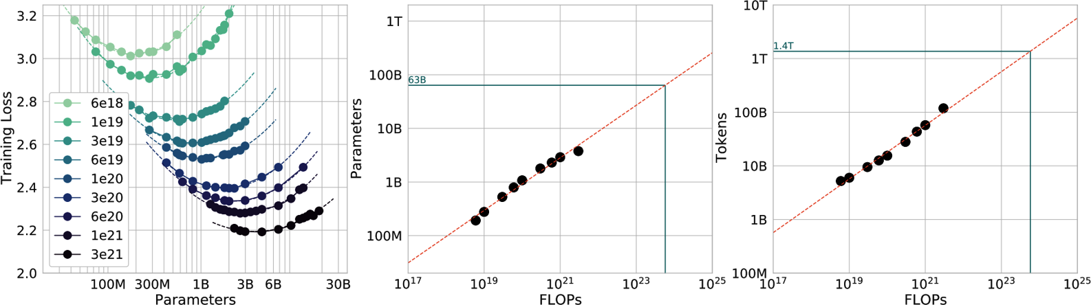
Figure 2-8. Graphs that depict the relationships between training loss, a model's number of parameters, FLOPs, and number of training tokens. Source: "Training Compute-Optimal Large Language Models" (DeepMind, 2022).
The scaling law was developed for dense models trained on predominantly human-generated data. Adapting this calculation for sparse models, such as mixture-of-expert models, and synthetic data is an active research area.
Some models, most notably Llama, have suboptimal performance but better usability. Given their compute budget, Llama authors could've chosen bigger models that would perform better, but they opted for smaller models. Smaller models are easier to work with and cheaper to run inference on, which helped their models gain wider adoption. Sardana et al. (2023) modified the Chinchilla scaling law to calculate the optimal LLM parameter count and pre-training data size to account for this inference demand.
On the topic of model performance given a compute budget, it's worth noting that the cost of achieving a given model performance is decreasing. For example, on the ImageNet dataset, the cost to achieve 93% accuracy halved from 2019 to 2021, according to the Artificial Intelligence Index Report 2022 (Stanford University HAI).
As Meta's paper "Beyond Neural Scaling Laws: Beating Power Law Scaling via Data Pruning" pointed out, this means a model with a 2% error rate might require an order of magnitude more data, compute, or energy than a model with a 3% error rate.
In language modeling, a drop in cross entropy loss from about 3.4 to 2.8 nats requires 10 times more training data. Cross entropy and its units, including nats, are discussed in Chapter 3. For large vision models, increasing the number of training samples from 1 billion to 2 billion leads to an accuracy gain on ImageNet of only a few percentage points.
Scaling Extrapolation
The performance of a model depends heavily on the values of its hyperparameters. When working with small models, it's a common practice to train a model multiple times with different sets of hyperparameters and pick the best-performing one. This is, however, rarely possible for large models as training them once is resource-draining enough.
This means that for many models, you might have only one shot of getting the right set of hyperparameters. As a result, scaling extrapolation (also called hyperparameter transferring) has emerged as a research subfield that tries to predict, for large models, what hyperparameters will give the best performance.
The current approach is to study the impact of hyperparameters on models of different sizes, usually much smaller than the target model size, and then extrapolate how these hyperparameters would work on the target model size.14 A 2022 paper by Microsoft and OpenAI shows that it was possible to transfer hyperparameters from a 40M model to a 6.7B model.
Scaling extrapolation is still a niche topic, as few people have the experience and resources to study the training of large models. It's also difficult to do due to the sheer number of hyperparameters and how they interact with each other. If you have ten hyperparameters, you'd have to study 1,024 hyperparameter combinations. You would have to study each hyperparameter individually, then two of them together, and three of them together, and so on.
To learn more about scaling extrapolation, check out this excellent blog post: "On the Difficulty of Extrapolation with NN Scaling" (Luke Metz, 2022).
Scaling Bottlenecks
Until now, every order of magnitude increase in model size has led to an increase in model performance. GPT-2 has an order of magnitude more parameters than GPT-1 (1.5 billion versus 117 million). GPT-3 has two orders of magnitude more than GPT-2 (175 billion versus 1.5 billion). This means a three-orders-of-magnitude increase in model sizes between 2018 and 2021. Three more orders of magnitude growth would result in 100-trillion-parameter models.15
How many more orders of magnitude can model sizes grow? Would there be a point where the model performance plateaus regardless of its size? While it's hard to answer these questions, there are already two visible bottlenecks for scaling: training data and electricity.
Training Data
Electricity
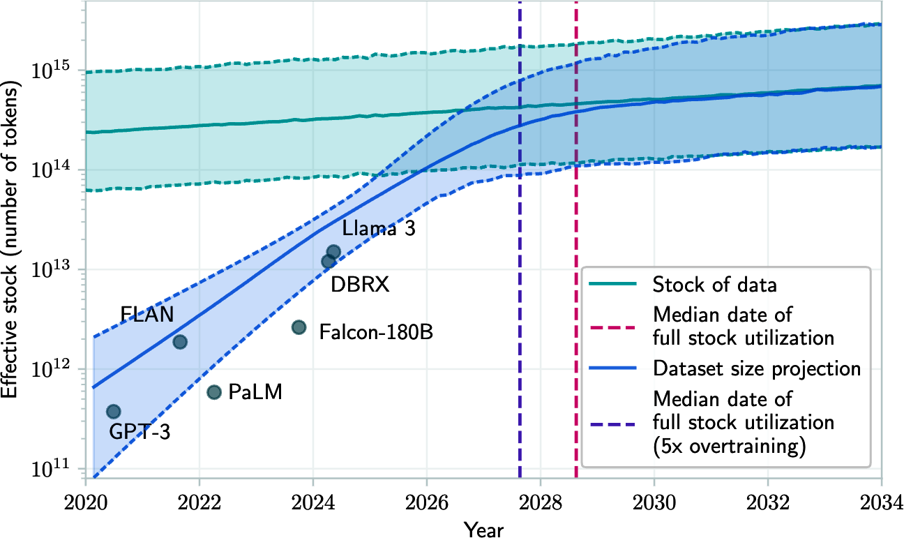
Figure 2-9. Projection of historical trend of training dataset sizes and available data stock. Source: Villalobos et al., 2024.
Some people are leveraging this fact to inject data they want into the training data of future models. They do this simply by publishing the text they want on the internet, hoping it will influence future models to generate the responses they desire. Bad actors can also leverage this approach for prompt injection attacks, as discussed in Chapter 5.
On top of that, the internet is being rapidly populated with data generated by AI models. If companies continue using internet data to train future models, these new models will be partially trained on AI-generated data. In December 2023, Grok, a model trained by X, was caught refusing a request by saying that it goes against OpenAI's use case policy. This caused some people to speculate that Grok was trained using ChatGPT outputs. Igor Babuschkin, a core developer behind Grok responded that it was because Grok was trained on web data, and "the web is full of ChatGPT outputs."16
Some researchers worry that recursively training new AI models on AI-generated data causes the new models to gradually forget the original data patterns, degrading their performance over time (Shumailov et al., 2023). However, the impact of AI-generated data on models is more nuanced and is discussed in Chapter 8.
Once the publicly available data is exhausted, the most feasible paths for more human-generated training data is proprietary data. Unique proprietary data -- copyrighted books, translations, contracts, medical records, genome sequences, and so forth -- will be a competitive advantage in the AI race. This is a reason why OpenAI negotiated deals with publishers and media outlets including Axel Springer and the Associated Press.
Until we can figure out a way to produce more energy, data centers can grow at most 50 times, which is less than two orders of magnitude. This leads to a concern about a power shortage in the near future, which will drive up the cost of electricity.
Now that we've covered two key modeling decisions -- architecture and scale -- let's move on to the next critical set of design choices: how to align models with human preferences.
Footnotes
- ML fundamentals related to model training are outside the scope of this book. However, when relevant to the discussion, I include some concepts. For example, self-supervision -- where a model generates its own labels from the data -- is covered in Chapter 1, and backpropagation -- how a model's parameters are updated during training based on the error -- is discussed in Chapter 7. ↩
- RNNs are especially prone to vanishing and exploding gradients due to their recursive structure. Gradients must be propagated through many steps, and if they are small, repeated multiplication causes them to shrink toward zero, making it difficult for the model to learn. Conversely, if the gradients are large, they grow exponentially with each step, leading to instability in the learning process. ↩
- Bahdanau et al., "Neural Machine Translation by Jointly Learning to Align and Translate". ↩
- Because input tokens are processed in batch, the actual input vector has the shape
N x T x 4096, where N is the batch size and T is the sequence length. Similarly, each resultingK, V, Qvector has the dimension ofN x T x 4096. ↩ - Why do simple activation functions work for complex models like LLMs? There was a time when the research community raced to come up with sophisticated activation functions. However, it turned out that fancier activation functions didn't work better. The model just needs a nonlinear function to break the linearity from the feedforward layers. Simpler functions that are faster to compute are better, as the more sophisticated ones take up too much training compute and memory. ↩
- Fun fact: Ilya Sutskever, an OpenAI co-founder, is the first author on the seq2seq paper and the second author on the AlexNet paper. ↩
- Ilya Sutskever has an interesting argument about why it's so hard to develop new neural network architectures to outperform existing ones. In his argument, neural networks are great at simulating many computer programs. Gradient descent, a technique to train neural networks, is in fact a search algorithm to search through all the programs that a neural network can simulate to find the best one for its target task. This means that new architectures can potentially be simulated by existing ones too. For new architectures to outperform existing ones, these new architectures have to be able to simulate programs that existing architectures cannot. For more information, watch Sutskever's talk at the Simons Institute at Berkeley (2023). ↩
- The transformer was originally designed by Google to run fast on Tensor Processing Units (TPUs), and was only later optimized on GPUs. ↩
- The actual memory needed is higher. Chapter 7 discusses how to calculate a model's memory usage. ↩
- Assuming a book contains around 50,000 words or 67,000 tokens. ↩
- As of this writing, large models are typically pre-trained on only one epoch of data. ↩
- FLOP/s count is measured in FP32. Floating point formats is discussed in Chapter 7. ↩
- As of this writing, cloud providers are offering H100s for around
$2to$5per hour. As compute is getting rapidly cheaper, this number will get much lower. ↩ - Jascha Sohl-Dickstein, an amazing researcher, shared a beautiful visualization of what hyperparameters work and don't work on his X page. ↩
- Dario Amodei, Anthropic CEO, said that if the scaling hypothesis is true, a
$100billion AI model will be as good as a Nobel prize winner. ↩ - AI-generated content is multiplied by the ease of machine translation. AI can be used to generate an article, then translate that article into multiple languages, as shown in "A Shocking Amount of the Web Is Machine Translated" (Thompson et al., 2024). ↩